Theoretical Background

The use of a high resolution crystal structure of the protein-ligand complex as the starting structure usually gives the most reliable and accurate model of the bound state, which is important for accurate simulation of the bound state. The application of the method to protein-ligand complexes obtained by docking or modeling the ligand binding mode by superposition is possible, but this usually requires longer equilibration times and more extensive sampling of binding poses.

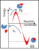
The residence time (\(\tau = 1 / k_\textrm{off}\)) of a complex is defined by the transition barrier energy (\(k_\textrm{off} \sim \exp \left(-\Delta G^\# \right)\)) and therefore depends on the characteristics of the bound (ground state - GS) as well as the transition (TS) states. Thus, simulation of the residence time requires sampling over the bound state (that defines affinity) and dissociation pathways.

 

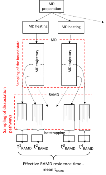
τRAMD provides an efficient simulation procedure for this purpose which is illustrated below. Specifically, several equilibration trajectories provide starting points for simulation of RAMD dissociation trajectories, while RAMD simulation of multiple dissociation trajectories from each starting point provides sampling of possible transition states. 

 

Required Software and Data

Software

1. Amber 14 tools and Sander for MD simulations
2. NAMD v11 
3. Python 2.7
4. R for statistical analysis
5. Pymol (or another visualization tool for ligand protonation)
6. VMD

 

Scripts and Input files

• Tutorial Instructions in PDF format
• You can download all the input files and scripts required to run this tutorial as a .tar file here.
• the latest version of the script for computing residence time can be also updated from here  tauRAMD.py

Type the following command to extract RAMD_tutorial_files_v2.tar in a directory called /home/ramd/ 

tar -xvf  RAMD_tutorial_files_v2.tar  -C  /home/ramd/

 

Description of the scripts and input files used during this tutorial

Preparation of the protein and ligand structures

complex.pdb – starting coordinates of the protein-ligand complex in PDB format

 

Generation of the topology and coordinate files for protein and ligand

tleap_ligand_in  - tleap input file for generation of the ligand parameters

tleap_all_in  - tleap input file for generation of the topology and coordinate files of the complex

 

Energy minimization, heating and short equilibration with restrains using AMBER

 amber_prep.sh

 

Heating and equilibration using NAMD

amber2namd_heating.in

amber2namd_equilibr.in

vmd_get-PDB.tcl

 

Simulation of dissociation using RAMD

RAMD-force.sh

 

Analysis of trajectories

bootstrapping.R

 

Procedure

Step 1:  Preparation of the protein and ligand structures

Partition the PDB format file (complex.pdb in our case) of the coordinates of the protein-ligand complex (without hydrogens added) into two files: protein (without hydrogens) and ligand (inhibitor is named as INH in complex.pdb file) using the UNIX grep command.

grep ^ATOM complex.pdb > protein.pdb

grep INH  complex.pdb > ligand.pdb

Protonate the ligand using pymol and save it as ligand_H.pdb; then remove all connectivity lines in the file.

• For protonation, load the ligand.pdb file into Pymol and click Action -> hydrogens -> add to add hydrogen atoms. Then save the molecule again as ligand.pdb (File -> Save molecule -> ligand -> OK). Instead of Pymol, another software (such as Chimera, Maestro Schrödinger, MOE) can be used. However, assignment of the protonation state is not always unambiguous and generally requires computation of pKa values. In the present case, the Pymol procedure is sufficient.

Select crystallographic water molecules within 5 Angstroms of the ligand, protonate them, and save them in the file water.pdb

• To select crystallographic water molecules, load the file complex.pdb into Pymol and type the following command in the Pymol command line utility: select resname HOH within 5 of resname INH
• This will create a selection named sele with water molecules within 5 Angstroms of the ligand. Then add hydrogen atoms to the selection (Action -> hydrogen -> add) and save the sele as water.pdb (File -> Save molecule -> sele -> OK)

Rename hydrogen atoms in the file water.pdb to make the atom naming scheme the same as for the protein (as the schemes are different in Amber and pymol):

sed "s/H01/H1 /"  water.pdb > water1.pdb

sed "s/H02/H2 /"  water1.pdb > water2.pdb

 

Step 2: Generation of protein and ligand parameters

Use the Amber tool antechamber to generate a mol2 format file from the pdb file of the ligand

antechamber -i ligand_H.pdb -fi pdb -o ligand_H.mol2 -fo mol2 -c bcc -s 2 -nc -1

• Antechamber generates a mol2 file that contains partial charges computed using the semiempirical BCC method  (see http://ambermd.org/antechamber/ac.html  for more details). The partial charges of the ligand can be also computed using the RESP web server (http://upjv.q4md-forcefieldtools.org/REDServer-Development/ ). Since the coordinates of the output mol2 file from the RESP web-server will differ from the original, this file cannot be used directly for simulations. Instead, the RESP partial charges from the mol2 file should be used to replace the partial charges of the ligand_H.mol2 file.

Use parmchk from Amber tools to determine the bond and atom types of the ligand (file INH.frcmod):

parmchk -i ligand_H.mol2 -f mol2 -o INH.frcmod

Use tleap from Amber tools to generate the ligand topology file, coordinate and pdb files  (INH.lib, INH.crd, INH.pdb):

tleap -f tleap_ligand_in

Combine the protein, ligand, and crystallographic water PDB files into one file in which  their coordinates are separated by TER lines:

grep ATOM protein.pdb > prot_lig.pdb

echo "TER" >> prot_lig.pdb

grep INH INH.pdb >> prot_lig.pdb

echo "TER" >> prot_lig.pdb

grep HOH  water2.pdb  >>  prot_lig.pdb

Solvate the system and add ions using tleap:

tleap -f tleap_all_in

which outputs topology (ref.prmtop), PDB (ref.pdb)  and coordinate (ref.impcrd) files in Amber format.

 

Step 3: Energy minimization, heating, and equilibration of the protein-ligand complex using Amber

sh amber_prep.sh

The output coordinate file ref-equil-NPT.crd will be used as an input for the next heating/equilibration step and in RAMD simulations.

 

Step 4: Heating and equilibration of the protein-ligand complex using NAMD

For sampling of the bound state in RAMD,  multiple starting points (i.e. NAMD restart files) usually need to be prepared.

• There are two strategies – either repeating the heating and equilibration steps several times (due to the random distribution in velocity assignment, each trajectory will be slightly different), or breaking the long equilibration run into parts and using intermediate states. These strategies can be combined to get better sampling. However, in the present example, we will prepare just one RAMD starting point for simplicity.

The input file for the heating procedure has to be adapted from the Amber output. Specifically, we have to convert the parameters of the simulation box from Amber to NAMD format. The Amber box parameters are stored in the last line of the minimized coordinate file ref-equil-NPT.crd​, for example​:

68.9465540  75.3446920  85.5960130  90.0000000  90.0000000  90.0000000

 

Place the first three numbers as cellbasisVector parameters in the NAMD input file  amber2namd_heating.in, as follows:

cellBasisVector1    68.9465540     0.   0.

cellBasisVector2    0    75.3446920       0.

cellBasisVector3    0                  0      85.5960130 

 

Then, check if the location of the topology ref.prmtop and coordinate ref-min.crd files for the heating and all equilibration files is correct. The correct path corresponding  to the location of ref.prmtop and ref-min.crd files must be specified in the input files.

Heat the system stepwise (10K steps, 200 ps in total) using a Langevin thermostat. The NAMD execution command depends on the system environment and options used for compilation. The simplest command is:

namd2 amber2namd_heating.in  > amber2namd_heating.out

Then equilibrate the system:

namd2 amber2namd_equilibr.in  > amber2namd_equilibr.out

Note that for equilibration, we use coordinates and velocities from restart files produced by the heating procedure.

Convert the equilibrated conformation to pdb format using the vmd script vmd_get-PDB.tcl as:

vmd -discdev text -e vmd_get-PDB.tcl -args amber2namd out

This script saves the last frame of the equilibrated trajectory into pdb format file (out.pdb) and compares this configuration corresponding to last frame (out.pdb)) with the starting configuration (ref.pdb). The script also generate files with RMSD values for protein and ligand across different frames of the trajectory with respect to the first reference frame.

Check if the location of the topology ref.prmtop file given in the  vmd_get-PDB.tcl script is correct

 

Step 5: Generation of the ligand dissociation trajectories using RAMD

Use the script RAMD-force.sh to prepare an input file for each trajectory in a separate directory and to execute NAMD. As in the previous step, edit the NAMD execution command at the end of the file to adjust it to the system environment. Check if the location of the tcl script for RAMD (RAMD-SCRIPT) is correctly described in the input file (see line “source  ./ RAMD-SCRIPT/ramd-4.1.tcl”  in the RAMD-force.sh file, the corresponding scripts, ramd-4.1_script.tcl, ramd-4.1.tcl, and vectors.tcl, are found in the NAMD distribution in the lib directory).

The first lines of the file should be adjusted to the particular system:

maxprot=4375  # the last atom in the protein structure

minlig=4376 # the first atom of the ligand structure

maxlig=4419 # the last atom in the ligand structure

molname=hsp90 # name used for the output file

force=14  # force to be applied

topfile=../ref.prmtop  # location of the topology file

rstfile=../ref-min.crd # location of the AMBER coordinate file after minimization

bincoor=../md_restart.coor # NAMD restat coordinate  file after equilibration

binvel=../md_restart.vel  # NAMD restat velocity  file after equilibration

xscfile=../md_restart.xsc # NAMD restat box parameter file after equilibration

 

Run the first trajectory as follows:

./RAMD-force.sh   101

Then repeat 9 more times with numbers 102 - 110

 

Step 6: Statistical analysis of the ligand dissociation trajectories

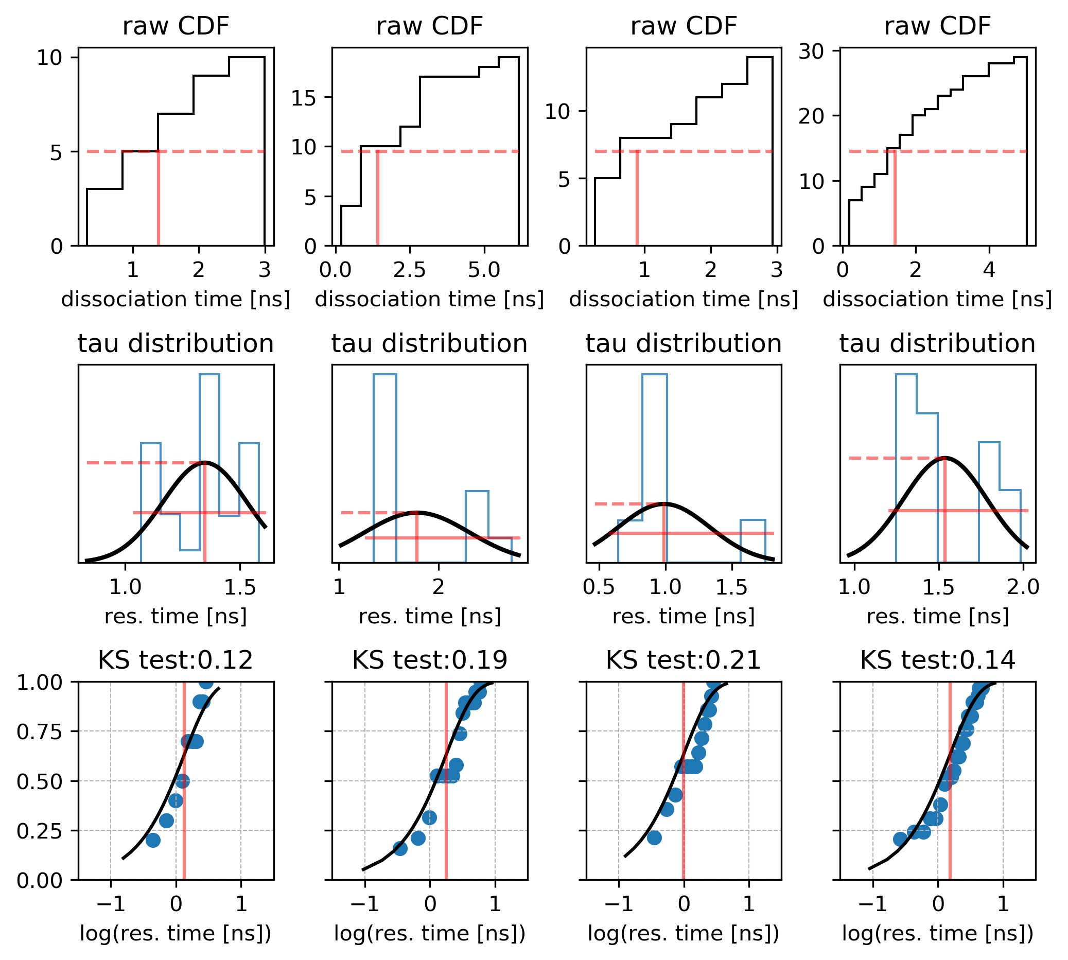
Extract the time when the ligand -protein distance reaches the maximum value (defined as 30 Angstroms in the RAMD input file) from each trajectory using the following command:

grep  "LIGAND EXIT EVENT DETECTE" */*out > times_1.dat

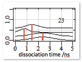
Plot the distribution of these times given in the times_1.dat file as a histogram. Ideally, the distribution should converge to an exponentially decreasing curve if there is only one dissociation route. The effective residence time is defined as the time when 50% of the trajectories have dissociated.

Use the bootstrapping method to derive the relative dissociation time from the trajectories generated by RAMD by running Rscript using the following command:

Rscript bootstrapping.R

(the bootstrapping.R script should be located in the same directory as times_1.dat )

The mean and standard deviation values printed in the standard output correspond to the relative residence time in ns and the standard deviation; the distribution of the relative residence times obtained from the bootstrapping procedure is stored in the file distribution.dat1

Running several sets of RAMD simulations starting from different equilibration points will provide a set of the residence time distributions, like this: