Data exploration and linear regression of a kinetic dataset using R
Summary
This tutorial guides the user through the process of doing multiple linear regression and data exploration on 16 p38 MAP kinase inhibitors with the software package R. Explorative data analysis is carried out on this dataset, containing precalculated physicochemical descriptors. Multiple linear regression and correlation analysis are utilized to identify descriptors influencing koff.
Requirements
- R >= 3.4
- R studio >= 1.1
- A csv file containing kinetic parameters of a congeneric series with precalculated physicochemical descriptors
R Packages
In addition the following R packages are needed for this tutorial.
The code snippet below installs all packages needed.
install.packages("cowplot", repos='http://cran.us.r-project.org')
install.packages("ggrepel", repos='http://cran.us.r-project.org')
install.packages("leaps", repos='http://cran.us.r-project.org')
install.packages("plotly", repos='http://cran.us.r-project.org')
install.packages("GGally", repos='http://cran.us.r-project.org')
install.packages("ggfortify", repos='http://cran.us.r-project.org')
Recommended literature
-
We recommend the excellent book R for Data Science by Hadley Wickham and Garrett Grolemund for a guided tour into R for Data Science.
-
For advanced classification and regression analysis, the R package caret developed by Max Kuhne is recommended. More on this topic
Format of the Input Dataset:
The input file has to be provided as a csv file. Each row represents a compound and the columns describe its physicochemical and kinetic parameters.
Sample File in this Tutorial
We extracted kinetic parameters for 16 MAP 38 alpha inhibitors from Regan et al. For these 16 inhibitors we calculated a set of five physicochemical descriptors using the MOE software. However any non-proprietary software can be used to generate the descriptors of interest, e.g. RDkit. This data is stored in the map38.csv file.
| column name | description |
|---|---|
| compound_key | compound identifier taken from Regan et al. |
| pkon | −log10 transformed kon value, as reported in Regan et al. |
| pkoff | −log10 transformed koff value, as reported in Regan et al. |
| pkD | −log10 transformed KD value, as reported in Regan et al. |
| vsa_positiv | postitive surface area; descr. Q_VSA_POS in MOE |
| vsa_negative | negative surface area; descr. Q_VSA_NEG in MOE |
| vsa_polar | polar surface area; descr. Q_VSA_POL in MOE |
| lipophilicity | lipophilicity; descr. logP(o/w) in MOE |
| weight | Molecular weight, Weight in MOE |
Download the provided map38.csv file on your computer and assign the file path to path_to_file. We then use the read.csv function to read the map38.csv file into R assign it to the map38 variable.
library(knitr)
# enter the local path to map38.csv file, e.g. /home/tutorial_user/K4DD/map38.csv
path_to_file = "map38.csv"
map38 <- read.csv(path_to_file)
# the head function shows you the first 6 rows of the map38 dataset
# knitr::kable is only used to format the output table and doesn't have to used
head(map38) %>% knitr::kable()
| compound_key |
pKD |
pkon |
pkoff |
vsa_positiv | vsa_negativ | lipophilicity | vsa_polar | weight |
|---|---|---|---|---|---|---|---|---|
| 2 | 10.01 | -4.93 | 5.08 | 369.66 | 183.17 | 4.94 | 147.38 | 527.67 |
| 3 | 5.92 | -5.07 | 0.85 | 204.59 | 125.31 | 2.97 | 81.18 | 306.80 |
| 5 | 10.01 | -5.19 | 4.82 | 342.38 | 193.22 | 4.64 | 147.38 | 513.64 |
| 6 | 8.23 | -4.81 | 3.42 | 315.11 | 193.22 | 4.29 | 147.38 | 499.61 |
| 7 | 7.80 | -4.40 | 3.40 | 371.93 | 190.94 | 3.74 | 180.42 | 543.67 |
| 8 | 7.64 | -5.16 | 2.48 | 357.09 | 125.24 | 2.99 | 170.62 | 451.57 |
Basic Data Exploration
library(knitr)
#knitr::kable() only used for table formatting and can be skipped
# once a library is load, it is not needed to use the prefix of the package (e.g. dplyr::, broom::, ...), however in this tutorial we will keep it to facilitate backtracing.
map38 %>%
dplyr::select(-compound_key) %>%
broom::tidy() %>%
dplyr::select(column, n, min, mean, max, range) %>%
knitr::kable()
| column | n | min | mean | max | range |
|---|---|---|---|---|---|
| pKD | 16 | 5.92 | 8.201875 | 10.01 | 4.09 |
| pkon | 16 | -5.19 | -4.517500 | -3.20 | 1.99 |
| pkoff | 16 | 0.85 | 3.685625 | 5.08 | 4.23 |
| vsa_positiv | 16 | 204.59 | 343.281250 | 459.19 | 254.60 |
| vsa_negativ | 16 | 125.24 | 173.359375 | 193.22 | 67.98 |
| lipophilicity | 16 | 2.97 | 4.463750 | 5.69 | 2.72 |
| vsa_polar | 16 | 57.94 | 143.048125 | 207.05 | 149.11 |
| weight | 16 | 306.80 | 489.707500 | 584.77 | 277.97 |
The pipe operator %>% is handy way to run a sequence of functions. The broom::tidy function provides us with a summary of the dataset. The dplyr::select function is used to select a set of columns, it can also be used to exclude columns using the "-" sign as a prefix, e.g. select(-compound_key)
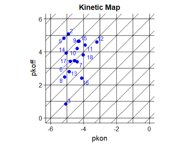
Kinetic map
Copy the code snippet below into R or R Studio. The output of this section is a kinetic map, plotting pkon values on the x-axis against pkoff values on the y-axis. This is a quick way to draw a kinetic map, using ggplot2 . It allows visual inspection of the kinetic data distribution and facilitates the detection of outliers. Values of xintercept and yintercept can be altered according to covered pkon and pkoff ranges.
library(cowplot)
library(ggrepel)
ggplot2::ggplot(map38, aes(x=pkon, y=pkoff)) + geom_point(size =3, color = "blue") +
geom_abline(intercept = 0:12, slope = 1) +
geom_hline(yintercept = 0:6) +
geom_vline(xintercept = 0:-6) +
geom_text_repel(aes(label = compound_key), color = "blue") +
coord_fixed() +
ggtitle("Kinetic Map")
ggplot2::geom_abline draws diagonal lines
ggplot2::geom_vline draws vertical lines
ggplot2::geom_hline draws horizontal lines
ggplot2::ggrepel::geom_text_repel is used to avoid olverlapping labels
Visualization of Data Distribution
Data Standardisation
The following code snippets provides a routine to standardise your data using scale.
library(knitr)
# The scale function returns a data matrix, however for further processing we need to convert it to a data.frame object which is achieved by the as.data.frame funtion.
map38_standardised <-
map38 %>%
dplyr::select(-compound_key) %>%
scale() %>%
as.data.frame()
# Gives you the first six rows of the standardised data frame.
map38_standardised %>%
head() %>%
knitr::kable()
| pKD | pkon | pkoff | vsa_positiv | vsa_negativ | lipophilicity | vsa_polar | weight |
|---|---|---|---|---|---|---|---|
| 1.6740729 | -0.7547556 | 1.2434457 | 0.3460330 | 0.4508013 | 0.5678886 | 0.0885297 | 0.4607009 |
| -2.1126997 | -1.0109151 | -2.5286925 | -1.8193335 | -2.2078841 | -1.7811728 | -1.2643874 | -2.2197076 |
| 1.6740729 | -1.2304803 | 1.0115885 | -0.0118225 | 0.9126020 | 0.2101635 | 0.0885297 | 0.2904373 |
| 0.0260398 | -0.5351903 | -0.2368733 | -0.3695467 | 0.9126020 | -0.2071824 | 0.0885297 | 0.1201736 |
| -0.3720805 | 0.2149910 | -0.2547085 | 0.3758105 | 0.8078353 | -0.8630118 | 0.7637621 | 0.6548718 |
| -0.5202183 | -1.1755890 | -1.0751263 | 0.1811414 | -2.2111006 | -1.7573245 | 0.5634813 | -0.4628246 |
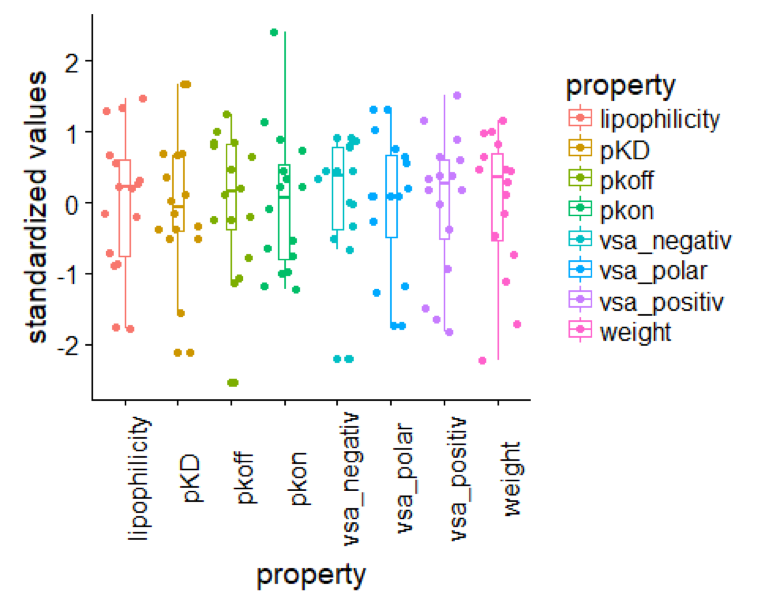
Box Plots
To prepare for the boxplot the data needs to be transformed using the tidyr::gather function. More on data transformation in R can be found here
library(ggplot2)
# data transformation, necessary for noxplot
trans_map38_standardised <-
map38_standardised %>%
tidyr::gather(key ="property", value = "standardized values")
# boxplot
ggplot2::ggplot(data = trans_map38_standardised, aes(x=property, y = `standardized values`, color = property)) +
geom_boxplot(width = .2) +
geom_jitter() +
theme(axis.text.x = element_text(angle = 90)) # formating of the x axis, labels are turned by 90?
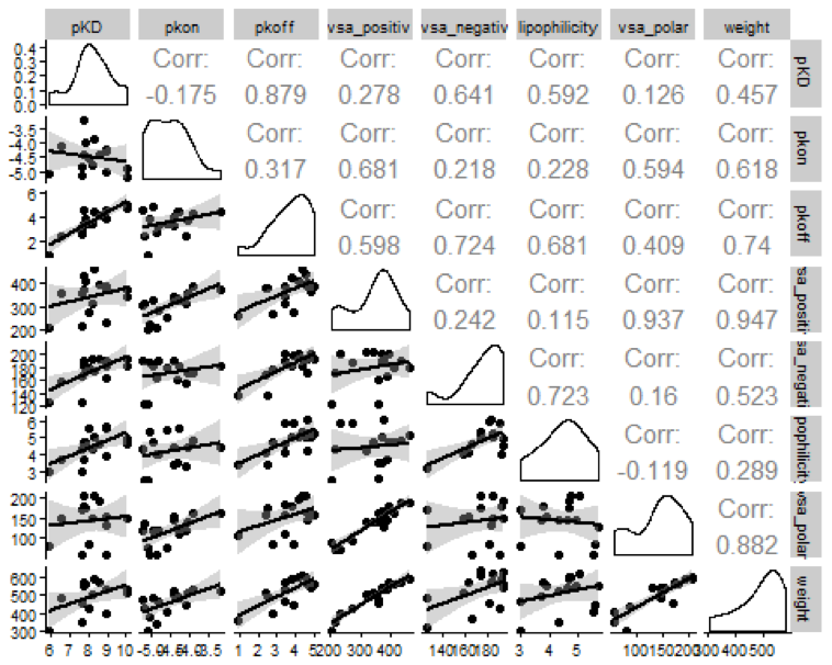
Structure Kinetic Relationships (SKR)
Scatterplot and Correlation matrix
A scatterplot matrix can be used to identify correlations between variables. The R package GGally provides the ggpairs function which outputs a scatterplot and correlation matrix from a data frame.
GGally::ggpairs(data=map38 %>% select(-compound_key), lower = list(continuous = "smooth")) +
cowplot::theme_cowplot(font_size = 8)
Multiple Linear Regression
Best Subset Selection
The leaps package includes the regsubsets function which provides forward, backward and exhaustive search for the best variable subset of a linear regression model. In this example we used the exhaustive method which tries all possible variable combinations. The output of the regbusbets function can be forwarded to the plot function, which sorts the variable combinations according to the adjusted R2.
map38_input <-
map38 %>%
dplyr::select(-pkon, -pKD, -compound_key)
#regsubsets
# methods = c("exhaustive", "backward", "forward")
regfit <- leaps::regsubsets(pkoff ~ ., data=map38_input, method = 'exhaustive')
plot(regfit, scale = 'adjr2')
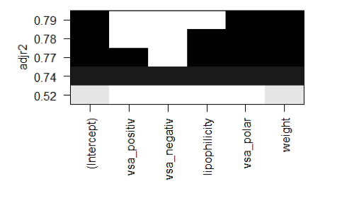
According to the regsubsets function the best variable combination for a linear model is vsa_polar and weight.
This combination yields in an adjusted R2 = 0.79.
Linear Regression Model
The R function lm returns a linear regression model. From the regsubsets function in the prior step, we found that weight and vsa_polar yielded in the best adjusted R2.
model %>% summary()
## Call:
## lm(formula = pkoff ~ vsa_polar + weight, data = map38)
##
## Residuals:
## Min 1Q Median 3Q Max
## -0.88454 -0.28028 0.01499 0.31944 0.68628
##
## Coefficients:
## Estimate Std. Error t value Pr(>|t|)
## (Intercept) -4.110366 1.036374 -3.966 0.001612 **
## vsa_polar -0.025235 0.005782 -4.364 0.000766 ***
## weight 0.023291 0.003433 6.784 1.29e-05 ***
## ---
## Signif. codes: 0 '***' 0.001 '**' 0.01 '*' 0.05 '.' 0.1 ' ' 1
##
## Residual standard error: 0.516 on 13 degrees of freedom
## Multiple R-squared: 0.8165, Adjusted R-squared: 0.7883
## F-statistic: 28.93 on 2 and 13 DF, p-value: 1.634e-05
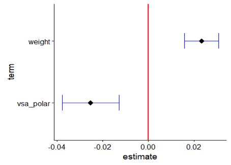
The model shows significant coefficients, however due to the strong intercorrelation between weight and vsa_polar one should be careful about interpretation. The ggcoef function can be used to visualize the coeffients of a regression model, including their standard errors.
GGally::ggcoef(model,
exclude_intercept = TRUE,
vline_linetype = "solid",
errorbar_height = .25,
vline_color = "red",
errorbar_color = "blue",
size = 4,
shape = 18
)
3D-Plot of Parameter Space
The plotly package allows the production of interactive 3D plots. The R code below is translated into HMTL and Javascript and thus enable interactive behaviour. Here, we created a point plot using the variables vsa_polar, weight and pkoff.
This plot can only be viewed in HTML mode and WebGL enabled browsers.
plot_ly(map38, x = ~weight, y = ~ vsa_polar, z= ~pkoff, text = ~paste('compound: ', compound_key)) %>% add_markers(color=~pkoff)
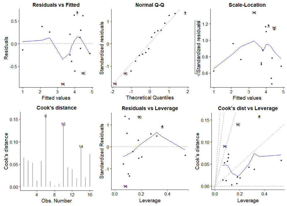
Regression Diagnostics
An excellent introduction on regression diagnostics can be found here. More on regression diagnostics in R. The stastistical significance tests for the coefficients and the regression model are based on assumptions of the underlying data and error terms. The ggfortify provides a set of diagnostic plots to evaluate our obtained regression model.
autoplot(model, which = 1:6, ncol = 3)