Generation of Quantitative structure-kinetics relationships (QSKRs) using Comparative Binding Energy (COMBINE) Analysis

Theoretical Background

Drug-binding kinetics, i.e. the rates at which a drug associates with (k_on) and dissociates from (k_off) the active site of its macromolecular target, constitute important early stage parameters for predicting the overall pharmacological effects of a drug in vivo. There has been growing consensus that optimizing the affinity alone under equilibrium conditions does not essentially translate into higher potency in vivo and instead the kinetic parameters (k_on and k_off) should be optimized to ensure better efficacy. Therefore, robust and high-throughput in silico methods are needed to predict kinetic parameters and mechanistic determinants of drug-protein binding. With the continual increase in the amount of measured experimental data on drug-binding kinetics and the number of crystallographic structures of ligand-receptor complexes resolved, approaches to derive 3D Quantitative-Structure-Kinetics relationships (QSKRs) offer considerable potential for predicting kinetic rate constants for new compounds. COMparative BINding Energy (COMBINE) analysis is one such approach. It can be used to derive a target-specific scoring function to compute binding free energy, drug-binding kinetics or a related property by exploiting the information contained in the 3D structures of receptor-ligand complexes.

 In COMBINE analysis, energy-minimized structures of protein-ligand complexes are used to compute protein-ligand interaction energies using a molecular mechanics force field. These energies are then partitioned and subjected to regression based methods such as Partial Least Squares (PLS) regression, to derive a statistical model which relates the predicted quantity to weighted selected components of the drug-receptor interaction energy. The interaction energy components are typically Lennard-Jones and Coulombic terms from a standard force field, decomposed on a per residue basis. If a sufficiently large number of molecules with known activities and 3D structures of ligand-receptor structures for these molecules are used in the training set, the weights of these interaction energy terms can be estimated by linear fitting. Due to the rather large number of interaction terms used in the linear fitting,  standard multiple regression techniques are not employed;  instead, partial least squares (PLS) analysis is applied to perform statistical analysis to determine the weights and the error coefficient C. 

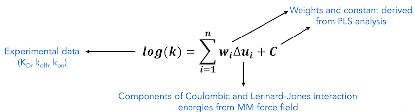
To perform COMBINE analysis, an energy matrix is generated where the columns represent each of these interaction energy terms (independent variables) and rows correspond to each ligand in the training set. The inhibitory activities or kinetics (dependent variable) of these ligands are added to the final column in the matrix. Then, the PLS method is used to maximize the linear correlation between the independent and the dependent variables by performing rotations of this matrix in the latent variables (LV) or the Principal Components (PC) space. In order to exclude energy terms that do not contribute to binding from the QSAR/QSKR, a variable selection procedure can be carried out. The variable selection procedure involves evaluation of the effects of each independent variable on the model predictivity and may be carried out iteratively using a combination of D-optimal and fractional factorial designs. However, in this work, instead of this variable selection procedure, we have used a pre-screening procedure where only those interaction energy terms that have standard deviation above a specified threshhold value were selected for PLS regression and the rest of the energy terms, showing little or no variance across the training dataset, were eliminated from statistical analysis. The main advantages of correlating inhibitory activity or kinetics (∆G, K_D, k_off , k_on, pKi , pIC₅₀ etc.) with residual interaction energy components over simply correlating with total computed binding energy is that the resultant COMBINE analysis model can help to highlight key interactions that are important to explain the observed variances in the biological activity. This information may also help in providing insights for predicting the effects of point mutations in proteins and for designing compounds with improved binding properties.

Required Software and Data

Software

1. Amber 14 tools for preparation of topology and coordinate files for protein-ligand complexes
2. PyMOL (or another visualization tool for ligand protonation)
3. gCOMBINE for performing COMBINE analysis

The source files for gCOMBINE can be downloaded from here

Data files

You can download all the data and input files needed to run this tutorial as a .ZIP file from the Supporting information of Gaurav K. Ganotra & Rebecca C. Wade, ACS Medicinal Chemistry Letters 2018.  (ml8b00397_si_002.zip (20.17 MB))

Type the following command to extract ml8b00397_si_002.zip into a directory called /home/combine/ 

unzip  ml8b00397_si_002.zip -d  /home/combine/

Description of the scripts and input files used during this tutorial

Preparation of the protein and ligand structures

complex.pdb – starting coordinates of a sample protein-ligand complex in PDB format

Generation of the topology and coordinate files for protein and ligand

tleap_ligand_in  - tleap input file for generation of the ligand parameters

tleap_complex_in  - tleap input file for generation of the topology and coordinate files of the complex

Energy minimization using AMBER

amber_prep.sh

Input file for COMBINE analysis

input_combine

Procedure

The steps 1 to 3 of procedure are optional and they guide the user on how to generate AMBER topology and coordinate files for their system of interest. For this tutorial, we will use the pre-prepared AMBER topology (hsp90_amber_topology_files.zip) and coordinate (hsp90_amber_coordinate_files.zip) files for 70 HSP90-inhibitor complexes. 

Step 1:  Preparation of the protein and ligand structures

Partition the PDB format file (complex.pdb in our case) of the coordinates of the protein-ligand complex (without hydrogens added) into two files: protein (without hydrogens) and ligand (inhibitor is named as INH in complex.pdb file) using the UNIX grep command.

grep ^ATOM complex.pdb > protein.pdb

grep INH  complex.pdb > ligand.pdb

Protonate the ligand using PyMOL and save it as ligand_H.pdb; then remove all connectivity lines in the file.

• For protonation, load the ligand.pdb file into PyMOL and click Action -> hydrogens -> add to add hydrogen atoms. Then save the molecule again as ligand.pdb (File -> Save molecule -> ligand -> OK). Instead of PyMOL, another software (such as Chimera, Maestro Schrödinger, MOE) can be used. However, assignment of the protonation state is not always unambiguous and generally requires computation of pKa values. In the present case, the PyMOL procedure is used for the sake of simplicity.

Step 2: Generation of protein and ligand parameters

Use the Amber tool antechamber to generate a mol2 format file from the pdb file of the ligand

antechamber -i ligand_H.pdb -fi pdb -o ligand_H.mol2 -fo mol2 -c bcc -s 2 -nc -1

• Antechamber generates a mol2 file that contains partial charges computed using the semiempirical BCC method  (see http://ambermd.org/antechamber/ac.html  for more details). The partial charges of the ligand can be also computed using the RESP web server (http://upjv.q4md-forcefieldtools.org/REDServer-Development/ ). In the publication, the partial charges of all the inhibitors were generated using the RESP approach.

Use parmchk from Amber tools to determine the bond and atom types of the ligand (file INH.frcmod):

parmchk -i ligand_H.mol2 -f mol2 -o INH.frcmod

Use tleap from Amber tools to generate the ligand topology file, coordinate and pdb files  (INH.lib, INH.crd, INH.pdb):

tleap -f tleap_ligand_in

Combine the protein and ligand PDB files into one file in which their coordinates are separated by TER lines:

grep ATOM protein.pdb > prot_lig.pdb

echo "TER" >> prot_lig.pdb

grep INH INH.pdb >> prot_lig.pdb

Generate topology and coordinate files for the protein-ligand complex using tleap:

tleap -f tleap_complex_in

which outputs topology (ref.prmtop), PDB (ref.pdb)  and coordinate (ref.inpcrd) files in Amber format.

Step 3: Energy minimization of the protein-ligand complex using Amber

The energy minimization procedure consists of four steps:  first with restraints on all protein and ligand heavy atoms (with force constants of 500, 50, and 5 kcal/mol A²) and then without restraints. The input files are prepared using the amber_prep.sh script and minimization is performed using the PMEMD module of Amber. Run the amber_prep.sh script through the command line as:

sh amber_prep.sh

The output coordinate file ref-min.crd will be used as an input for performing the COMBINE analysis as it contains the coordinates for the Amber minimized complex.

Follow the above steps 1 to 3 for all the protein-ligand complexes to be used for performing COMBINE analysis.

Step 4: Download data files for performing COMBINE analysis

You can download all the data and input files needed to run this tutorial as a .ZIP file from the Supporting information of Gaurav K. Ganotra & Rebecca C. Wade, ACS Medicinal Chemistry Letters 2018.  (ml8b00397_si_002.zip (20.17 MB))

Type the following command to extract ml8b00397_si_002.zip into a directory called /home/combine/ 

unzip  ml8b00397_si_002.zip -d  /home/combine/

The above command will generate the following 5 files in the directory: /home/combine/supplementary_files/

1. hsp90_energy_minimized_pdb_files.zip  : This zipped file contains 70 energy-minimized structures of N-HSP90-inhibitor complexes in PDB format.
2. hsp90_amber_topology_files.zip :  This zipped file contains 70 topology (.top) files for N-HSP90-inhibitor complexes generated by the LEaP program of Amber 14 using ff14SB and GAFF force fields for the protein and inhibitors, respectively. These topology files are required for performing the PLS analysis with the gCOMBINE program.
3. hsp90_amber_coordinate_files.zip :  This zipped file contains 70 coordinate (.crd) files for N-HSP90-inhibitor complexes generated by the LEaP program of Amber 14 and they are also required by the gCOMBINE program.
4. hsp90_gCOMBINE_output_models.zip :  This zipped file contains the output of 3 different COMBINE models generated in this publication using the gCOMBINE program. These files can be directly loaded into the gCOMBINE program (using the Load model option) to visualize the results of PLS analysis. We, however, do not require these pre-prepared models for this tutorial as we will be generating the COMBINE analysis model using the input file (input_combine) for gCOMBINE program.
   • hsp90_output_model_koff  :  COMBINE analysis model generated for k_off rates of HSP90 inhibitors.
   • hsp90_output_model_KD   :  COMBINE analysis model generated for K_D (binding affinity) of HSP90 inhibitors.
   • hsp90_output_model_KD_resorcinol  :  COMBINE analysis model generated for K_D (binding affinity) of resorcinol class of HSP90 inhibitors.
5. Nomenclature_files.xlsx  :  The nomenclature of the PDB, coordinate and topology files for the protein-inhibitor complexes provided in the zipped files above is different from the nomenclature of the inhibitors used in the manuscript. This Excel spreadsheet provides the mapping between the inhibitor names mentioned in the manuscript and their corresponding file names in the zipped folders. We however, do not require this Excel spreadsheet for this tutorial.

For the subsequent steps, we will only be using the already prepared AMBER topology (hsp90_amber_topology_files.zip) and coordinate (hsp90_amber_coordinate_files.zip) files for energy-minimized 70 HSP90-inhibitor complexes.

Step 5:  Copy Amber topology (.top) and coordinate (.crd) files for all energy-minimized complexes into a directory

Extract topology and coordinate files for all the 70 energy-minimized complexes in /home/combine/ directory.

cd /home/combine/supplementary_files/

unzip  hsp90_amber_topology_files.zip -d  /home/combine/

unzip  hsp90_amber_coordinate_files.zip -d  /home/combine/

Then create an empty directory to perform COMBINE analysis and copy all the topology and coordinate files to this directory.

mkdir /home/combine/run_combine

cp /home/combine/topology_files/* /home/combine/run_combine/.

cp /home/combine/coordinate_files/* /home/combine/run_combine/.

Step 6: Download the gCOMBINE software

The source files for gCOMBINE (gCOMBINE.zip) can be downloaded from here

Type the following command to extract gCOMBINE.zip in a directory called /home/combine/ 

unzip  gCOMBINE.zip -d  /home/combine/

Note: Do not forget to change the permissions to allow the user to read and execute the files/programs in the gCOMBINE directory and its underlying subdirectories by:

chmod -R 777 gCOMBINE/

Step 7:  Perform COMBINE analysis

Move to the run_combine directory:

cd /home/combine/run_combine/

Copy the input file for COMBINE (input_combine) to the run_combine directory:

cp input_combine /home/combine/run_combine/.

Run the gCOMBINE executable. The following command will open the gCOMBINE GUI.

java -jar /home/combine/gCOMBINE/bin/gCOMBINE.jar

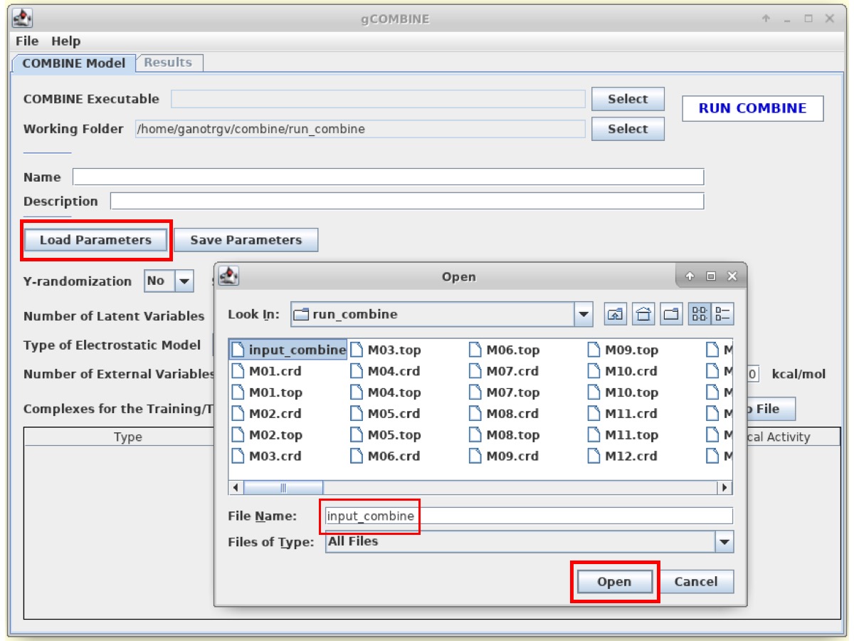
Click on Load Parameters and open the input file (input_combine).

Note:

The input file consists of information such as a list of input parameters used for running COMBINE analysis, file names of topology and coordinate files of complexes to be used, pharmacological activities (log(k_off) values in our case) of ligands, information on whether the complex is part of training dataset or test dataset etc. The 'file-format' for the standalone COMBINE input file is specific to the gCOMBINE program. In this tutorial, we are using the list of parameters that were optimized for this model. However, the user has the option to modify the input parameters for COMBINE analysis in the gCOMBINE interface to be specific for their system/activity of interest, and can save a valid standalone COMBINE input file using the Save Parameters button. For information on the list of different options/parameters (such as data scrambling, Scaling of variables, Number of Latent variables, Electrostatic models, External variables, Treatment of positive energies etc.) that are available for COMBINE, please refer to the documentation of the gCOMBINE program.

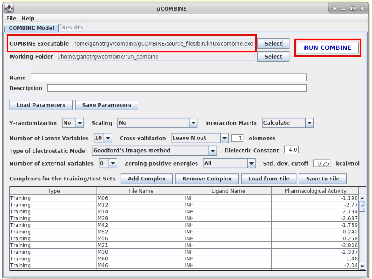
Now, enter the path of the COMBINE Executable to /home/combine/gCOMBINE/bin/linux/combine.exe

The user can also define the name for the model and its brief description. However, this step is OPTIONAL.

Then, click on RUN COMBINE button to run COMBINE analysis. The program will take few seconds/minutes to perform the COMBINE analysis.

Results:

The results for COMBINE analysis can be visualized under the Results tab at the top. 

gCOMBINE provides a summary for each principal component (latent variable) with the values for the correlation coefficients on both training and test datasets (if provided), and the errors (root mean squared error, average absolute error) between predicted and experimental values on training and test datasets (if provided). This summary is presented in a table and is also graphically displayed in a plot.

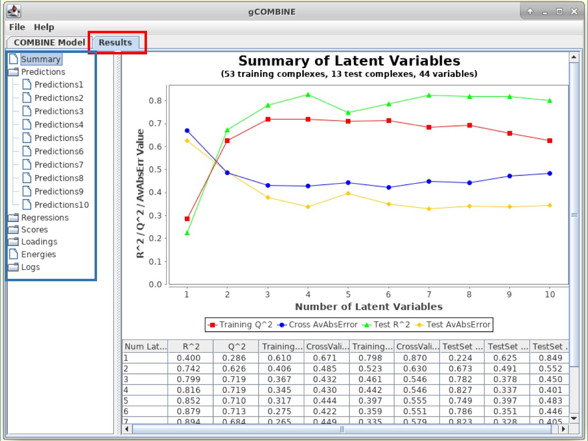
In the panel on the left-side of the Results window, there are several Buttons which display additional information such as:

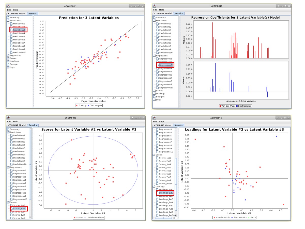
1. Predictions  This section displays plots of predicted versus experimental values for each latent variable. The diagonal straight line in the plot helps the user to observe the deviations between predicted and experimental values.

2. Regressions  The PLS regression coefficients of the energy variables are displayed for different numbers of latent variables. The top section of the plot displays the regression coefficients of the van der Waals interaction energies and the bottom section corresponds to the electrostatic interactions.

3. Scores  This section displays plots of the complexes in the space defined by two successive latent variables (score plot). The values of the scores can be understood as the values of the compound in the new variable space, the principal component space, and since this new space is normalized with zero mean, compounds lying far from the origin have values significantly deviating from the mean, and may therefore be outliers.

4. Loadings  This section displays the loading plots which describe the relation between the original variables and the new orthogonal latent variables by plotting the contributions of the calculated energy descriptors to two successive latent variables. These plots show the relations between the variables. For example, variables lying close together far from the origin may be correlated.

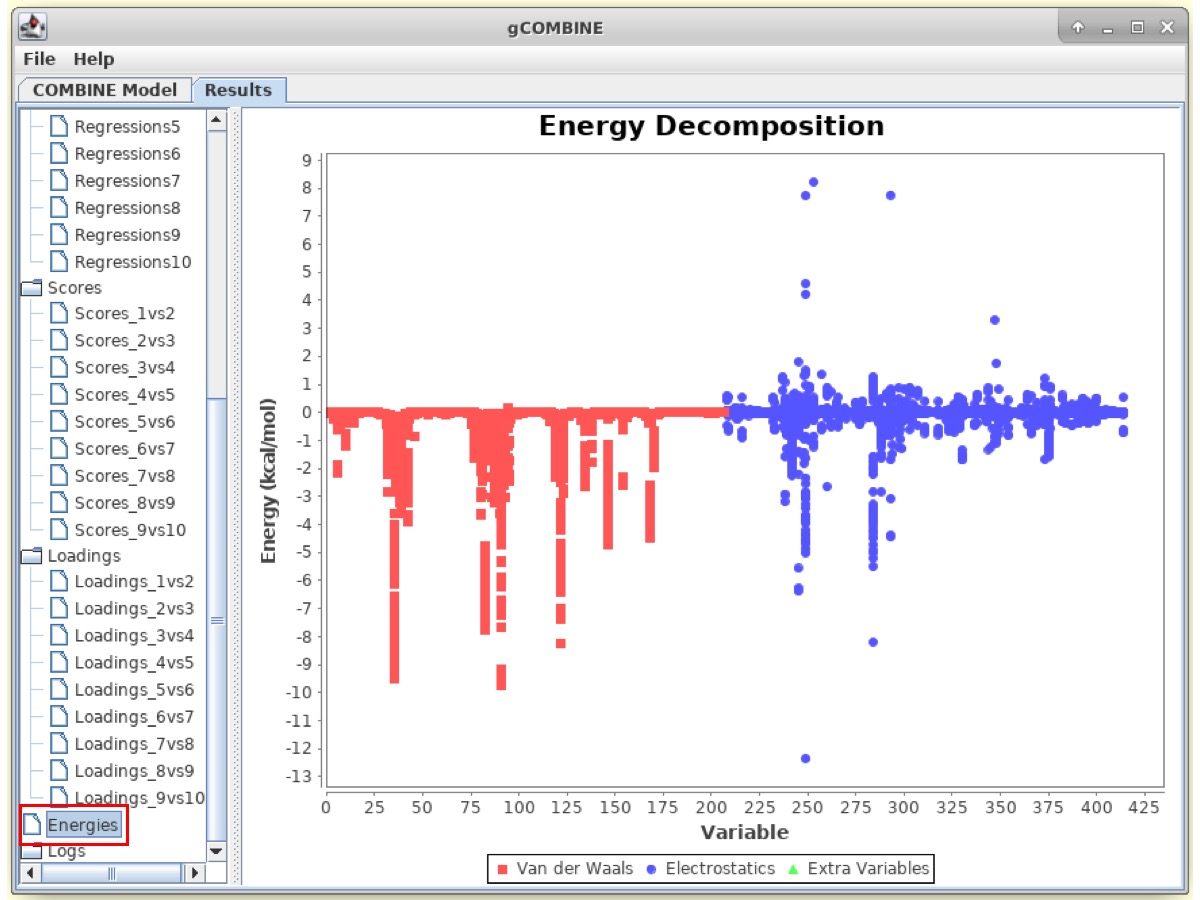
The Results window also displays information about the original energy values that are calculated in the force field and enter the PLS analysis. The plot displays van der Waals and electrostatic interaction energy values for different ligand-residue interactions for each complex. This plot can be useful to identify modeling errors resulting in anomalous energy values and also to visualize the range of energies in a particular ligand-residue interaction within a set of complexes.

Observe the correlation coefficients for regression (R²) and cross-validation (Q²) and errors between predicted and experimental values on the training and test datasets.

Try to change the type of Cross-validation in the COMBINE Model window to Leave 2 out or Leave 3 out and rerun the COMBINE analysis. Observe how the Q² values change for different numbers of latent variables and check the robustness of the model.