Compartmental modelling and simulation in Berkeley Madonna
Summary
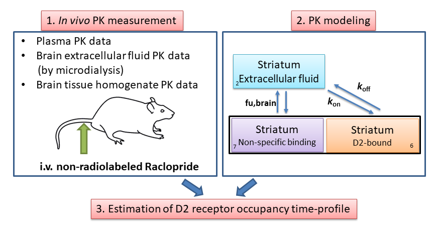
The aim of this tutorial is to demonstrate the use of compartmental modelling and simulation in Berkeley Madonna in predicting the receptor occupancy time profile in a body tissue after intravenous administration of a receptor ligand. In this tutorial, the selective dopamine D2 antagonist raclopride is used as an example. The pharmacokinetics (PK) and dopamine D2 receptor occupancy (RO) in brain after intravenous administration of raclopride to rat are simulated.
Theoretical Background
The concept receptor occupancy is defined as the fraction (%) of a receptor population that is occupied during treatment with a receptor ligand. Our goal is the simulate the in vivo receptor occupancy time profile after intravenous administration of a receptor ligand. To that end, we first need to have some ideas about the ligand concentration time profile in the body (i.e. PK), particularly at the target tissue where the receptor resides. Once we have information regarding the PK then we can construct a compartmental model to describe the ligand distribution time course in different body compartments including the target tissue. The receptor occupancy time profile can then be simulated by linking the PK profile at the target tissue to the ligand-receptor binding affinity constant (Kd) or binding kinetics (kon and koff). The following figure shows the general concept for simulating the receptor occupancy time profile based on compartmental PK modelling.
List of the tools/software used
Berkeley Madonna v8.3.23 (https://www.berkeleymadonna.com/)
- Used for constructing mathematical models (differential equations) and for plotting the simulated time profiles of drug concentration and drug effects (such as receptor occupancy). Proprietary license. A trial version of the software can be downloaded free, but the models cannot be saved, and the graphs and tables cannot be saved or copied.
- For tutorials and examples of using Berkeley Madonna in PK/PD modelling, the audience can refer to the following:
- A Krause and P J Lowe. Visualization and Communication of Pharmacometric Models With Berkeley Madonna. CPT Pharmacometrics Syst Pharmacol. 2014; 3(5): e116. http://onlinelibrary.wiley.com/doi/10.1038/psp.2014.13/abstract
- W-S Park. Pharmacometric models simulation using NONMEM, Berkeley Madonna and R. Transl Clin Pharmacol. 2017;25(3):125-133. ref
Input script used in the tutorial
1. Berkeley Madonna code
- Berkeley Madonna code for simulating PK and D2 occupancy of raclopride in rat brain.mmd – Once opened using Berkeley Madonna you can see all the codes and mathematical equations used to construct the PK-RO model.
Download the Berkeley Madonna code required for this tutorial here
Procedure
Step 1: Obtaining PK information of the receptor ligand
In our raclopride example, the PK data in plasma and brain (target tissue) were obtained from an in vivo PK experiment in rat.
Step 2: Designing the structure of the compartmental PK model
The structure of the compartmental PK-RO model for raclopride in rat is shown in the figure 2. In general, there are one central compartment to describe the ligand concentration in plasma, one or two peripheral compartment(s) to describe the ligand distribution to non-target tissues, and one target compartment to describe the ligand distribution to the target tissue.
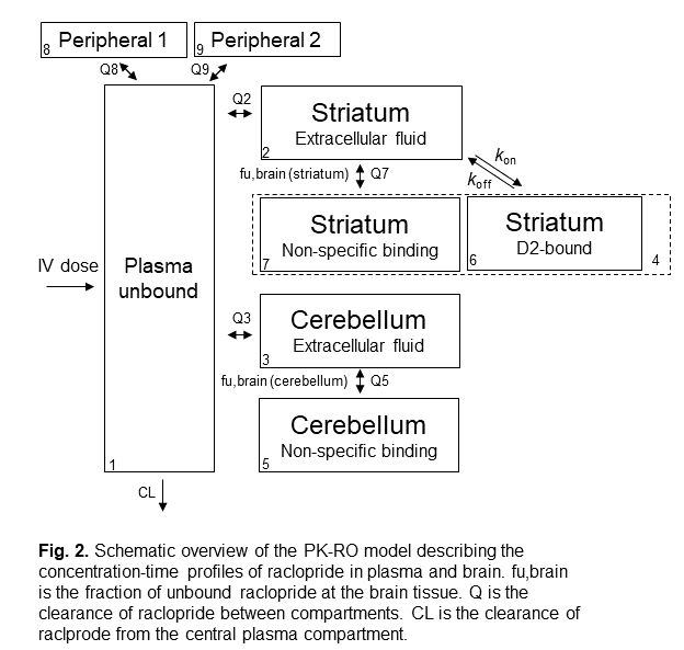
In our raclopride example, the target tissue is the striatum tissue in brain (which is the tissue with high D2 receptor density). The cerebellum tissue in brain serves as a reference tissue (which is a tissue with negligible amount of D2 receptor, so it reflects the non-specific tissue binding of raclopride to brain tissue).
Step 3: Drafting the differential equations of the compartmental PK model
Differential equations are drafted to describe the change in the amount (not concentration) of the ligand at different time in different compartments. In general, the concept is that the change in the amount of ligand in a compartment equals to the total input rates minus the total output rates. For example, for a two-compartment model the change in the amount of ligand in compartment 1 (A1) can be something like:
where K12 and K21 are the first-order clearance rate of the ligand from compartment 1 to 2 and from 2 to 1, respectively.
Step 4: Estimating the PK-related parameters of the compartmental PK model
In our raclopride example, a population PK analysis was performed using a non-linear mixed effects modeling approach, which estimates the typical (mean) value of model parameters as well as their inter-individual variances using the software NONMEM® (version 7.3.0, ICON). There are other non-linear mixed effects modeling software such as Monolix (Lixoft) and Phoenix NLME (Certara). While all the above software require a paid license, there are also packages in R that are free, for example nlmeODE .
Step 5: Linking receptor occupancy to the compartmental PK model to form the PK- receptor occupancy model
There are two possible approaches, depending on the binding kinetics data we have:
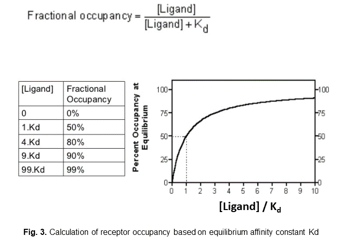
1. if we only have the equilibrium affinity constant (Kd) data, then we can use the equation shown in the figure 3:
(assumption: the ligand-receptor binding reaches equilibrium instantaneously)
When ligand concentration is equal to Kd, then receptor occupancy is 50%.
2. if we have data regarding the ligand-target association rate (kon) and dissociation rate (koff), then we can use the following equation:
(assumption: the ligand-receptor binding is a one-step process)
where:
“LR complex amount” is the amount of ligand-receptor complex;
“available receptor amount” is the amount of non-occupied receptor that is still available for ligand binding. It is calculated as the total amount of receptor (Bmax) minus the amount of receptor already bound to ligand (“LR complex amount”); and
[ligand] is the concentration of free ligand at the tissue.
Receptor occupancy is then calculated as:
Step 6: Perform simulation to simulate the PK and receptor occupancy-time profiles at the target tissue
To generate a simulation, input the desired dosing information such as:
IV dose of raclopride: in the example it is “doseperkg = 6” which means a raclopride dose of 6 nmol/kg of body weight of the rat
Body weight of the rat: e.g. bw = 0.25 (kg)
IV infusion time: the duration of the IV infusion. If it is a bolus injection as in the example, then we set the infusion time to a small value, e.g. “infusetime = 0.1” (0.1 min)
Once the dosing information is set, press “Run”.
Simulated amount-time profiles in different compartments will be generated in a new plot. (as mentioned in Step 3, the differential equations in the model describe the change in the amount (not concentration) of the ligand. Therefore, the default simulation plot displays the amount of ligand instead of concentration of ligand)
To generate concentration time profile and receptor occupancy time profile, select the “Graph” tab and select “Choose Variables”. At “Choose Variables” you can pick the variables (PK and/or receptor occupancy) that you would like to simulate.
Press “Run” again to generate a new plot which displays the selected variables.
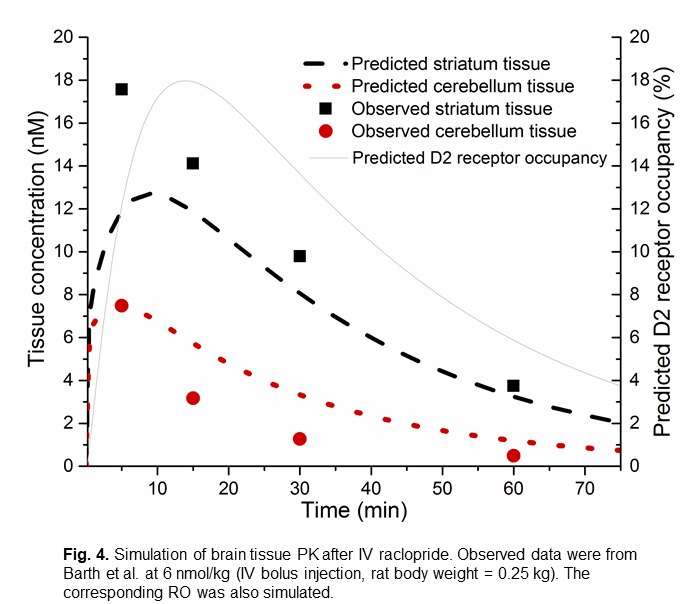
The figure 4 is an example of simulated brain tissue PK and striatum D2 receptor occupancy after IV raclopride. The simulated brain tissue PK matches the observed values reported by Barth et al. (2006).
Step 7: Extra: Performing simulation to investigate the impact of different parameters on the PK / RO outcomes
The Berkeley Madonna software allows easy visualization of the change in PK-RO profile when a parameter of the model changes.
At the “Parameters” tab, select “Define Sliders”. Then you can select the parameters and the corresponding range of the values that you would like to test. A box of sliders will appear. When you change the value of a parameter using the slider, the simulation plot will be updated. You can use it to simulate the change PK-RO profile when the condition changes. For example:
- different doses
- different infusion durations
- different ligand elimination rates from the central plasma compartment
- different binding kinetics (kon, koff, Kd)
References
- Barth, V.N., Chernet, E., Martin, L.J., Need, A.B., Rash, K.S., Morin, M., Phebus, L.A., 2006. Comparison of rat dopamine D2 receptor occupancy for a series of antipsychotic drug measured using radiolabeled or nonlabeled raclopride tracer. Life Sci. 78, 3007-3012. [this was a rat study which reported brain tissue PK after IV raclopride injection as shown in the figure in step 6.
- Wong Y.C., Ilkova T., van Wijk R.C., Hartman R., de Lange E.C.M., 2018. Development of a population pharmacokinetic model to predict brain distribution and dopamine D2 receptor occupancy of raclopride in non-anesthetized rat. Eur. J. Pharm. Sci. 111, 514-525.